“I used to think if there was reincarnation, I wanted to come back as the president or the pope or a .400 baseball hitter. But now I want to come back as the bond market.”
                                                                                         James Carville (campaign advisor to President Bill Clinton, 1993)

Times were very different when James Carville was grousing about the dominance of the bond market, but his point remains true today: the stock market gets the headlines, but when it comes to understanding what’s going on in the economy and corporate America, you’ve got to look to the bond market. 

The COVID-19 pandemic has triggered an economic and social crisis, the likes of which have not been seen for a century.  Prices and other signals from bonds sold by companies and financial institutions in the “corporate” bond market speak to the risks of company survival, a baseline necessity for economic recovery, in ways that equities do not.  This blog will focus on analyzing the corporate bond market and its signals, with the aim of providing readers with fresh insights into the impact of the pandemic and the outlook for the US economy’s emergence from its deep slump. 

To date the corporate market’s headline message is that the pandemic’s impact will be significant, but not catastrophic.  But as I discuss below, the market’s signals have been distorted by the Federal Reserve Bank’s actions to support the market and ensure liquidity, something that is clear from a comparison with equity market metrics.  And as with any market analysis, there’s also the question of what’s priced into current levels.  Following the recent market rallies, the concern in this regard is whether investors are taking too rosy a view of the path forward.  (Spoiler alert: I think this is the case.)
​

Companies depend on the bond market to raise funds, and their reliance on it has increased due to the shrinking role of banks since the 2008-2009 financial crisis.  So when the market is severely disrupted, many firms will not survive for long.  Not so for the equity market, where the money flows the other way: over the past decade companies have paid out a lot more to investors via stock buybacks than they have received from selling new shares.  Thus, counterintuitive as it might sound, for most companies the gyrations of the stock market have little or no impact on their day to day operations. 

Another reason to pay close attention to corporate bonds is that their prices are closely aligned with company survival.  Declines in bond prices, particularly for riskier companies, are strong indications of an increased risk of bankruptcy - by definition an existential threat to them, and one with severe knock-on effects for workers and the economy.  By contrast, the relationship between most entities’ share prices and their risk of bankruptcy is tenuous at best.  A risky company’s shares can skyrocket if it has excellent growth prospects, while at the opposite end of the spectrum firms that are quite safe, but that are in stodgy industries (think electric utilities), typically have underwhelming equity performances. 

Before delving into an analysis of corporate bond market signals, to ensure that all readers are on the proverbial same page in the next section I provide a brief review of corporate bond basics for those in need of one.  
​

,When it comes to the corporate bond market, one of the key concepts is the credit spread (or simply, “the spread”).  This is the extra compensation that investors require to buy a corporate bond, with its attendant risk of default, instead of a comparable government security which (presumably) has no default risk.  (“Default” in the bond market is commonly defined as the failure of the company that sold the bond to pay, on time, the coupon amounts and repay the face value, or the principal, of the bond.)

Let’s take as an example a corporate bond with a yield of 7%.  A bond’s yield is the expected annual total return that an investor receives for holding it.  The total return has two components: 1) coupon payments to the bondholder, expressed as a percent of the bond’s original value; and 2) a portion of the difference between the market price of the bond and its face value, i.e., the amount that will be repaid to the investor when the bond matures.  If a government bond with the same maturity date as our corporate bond has a yield of 2%, then the corporate bond’s spread is 5% (7%-2%). 

So how do changes in investors’ perceptions of default risk feed through to changes in the interrelated bond metrics of spreads, yields, and prices?   

Spreads, especially for riskier companies, move in line with investors’ perception of default risk: when it rises, spreads go up.  Since a bond’s spread is a component of its yield, a higher spread means a higher yield.  For reasons that aren’t worth going into here, bond yields and prices move in opposite directions – an increase in a bond’s yield leads a drop in its price, and vice versa.  This is an important relationship, because while spreads are a key signal of default risk, investors buy and sell bonds on a price basis.  But the two metrics get you to the same place, in that increased default risk results in both higher spreads and lower prices.  

A final point is that since default is a future event that may or may not happen, any estimate of it for a given company is just that – an estimate or, less politely, a guess.  In the world of corporate bonds, credit ratings from agencies such as Moody’s, Standard & Poor’s, and Fitch provide a common shorthand for estimates of default risk.  Bonds with low estimated default risk are termed investment grade and have ratings of Baa3/BBB- and above.  As lower risk securities, they tend to have lower credit spreads and thus lower yields.  Issues with low ratings (Ba1/BB+ and below) usually have higher spreads and yields and are classified as high yield, speculative grade, or junk bonds.  
​

With these preliminaries out of the way, we can now turn to corporate bond market signals.  Spreads on investment grade and high yield bonds rose sharply when the scale of the pandemic became evident, with the latter reacting more strongly than the former (Figure 1).  They have now partly recovered for reasons I discuss in the next section.
 
                      Figure 1: Investment Grade and High Yield Spreads (through April 22, 2020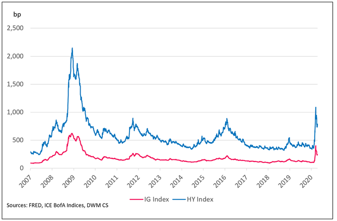

But despite the catastrophe facing the economy and millions of workers, at its peak the average high yield spread did not risen by nearly as much as during the 2008-2009 financial crisis.  One reason is that the current crisis is different from the last one: during the financial near-meltdown the credit markets were at the heart of the disaster, so it’s not surprising that a credit-focused metric like the average high yield spread blew out.  This time around, the corporate bond market is more in the position of suffering collateral damage from an exogenous event.

A second reason for the relatively limited spread widening is the one we stated at the outset, namely the Fed’s programs to support the markets, including buying investment grade and high yield bonds.  These moves have supplied crucial liquidity to the market and raised investors’ hopes that a financial catastrophe can be avoided.  This is highly significant in market terms, since a meltdown would block companies from selling debt and trigger a wave of defaults.  However, ensuring functioning bond markets is a different, and arguably easier, matter than avoiding a deep and long-lasting recession.  The unprecedented nature of the crisis, particularly its sudden and severe impact on individuals and small businesses, makes me think that we’ll achieve the first (relatively) happy outcome, but I’m far less sanguine about the second.  
​

(In addition to the Fed’s liquidity programs, the bond and equity markets have been supported by various Federal packages to aid workers and companies.  We now consider their impact as well, and assess the degree to which the bond markets have benefited disproportionately.

 Figure 2 shows the average high yield spread and the VIX Index of S&P 500 option volatility.  The VIX, commonly called the “fear index”, is used by equity investors to hedge against market declines, so it typically moves inversely to stocks.  Since the VIX captures the level of risk aversion amongst equity investors, it provides a good analog to a risk-sensitive bond metric like high yield spreads.  Reflecting this, the correlation coefficient of the time series is 80%.  Notably, they even tracked each other closely during the credit markets-centered financial crisis.  This makes the recent breakdown of the relationship, with the VIX shooting up by a much greater amount than the high yield spread, and then recovering sharply, all the more noteworthy.  I believe that there are two drivers of this divergence. 

                Figure 2: The average high yield spread and the VIX Index  (through April 22, 2020)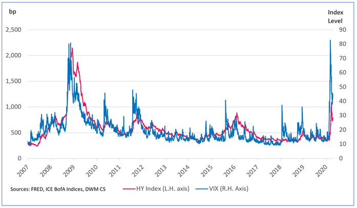

Firstly, as noted the Fed’s actions indeed helped, and will continue to help, the corporate bond market. This has contained the spread widening and underpinned the recent rally. Crucially, it has muted the signals concerning default risk that would have otherwise come from high yield spread levels.  It’s impossible to say by how much, but it would seem to be a significant amount.  The comparison with 2008 is tells us that much. 

The second factor in the divergence between the VIX and high yield spread is the varying impact of the economic support packages passed by Congress.  To be clear, equity investors and bondholders alike want to see companies survive and prosper, so the government’s actions are positive for both markets. However, share prices are usually more volatile than bond prices, mainly because shareholders have more upside and downside than bondholders. This likely contributed to  the VIX Index’s extreme moves compared to the high yield index, which hadn’t risen by as much in the first place, at least partly because of the aforementioned support provided by the Fed.

The VIX index is now back to around the same level as during the first quarter 2016 oil price collapse, while the high yield spread index is under it. This is noteworthy, since in many ways the events of 2016 were much less serious than the challenges we're facing today.  For the bond markets, a good part of the recovery is due to investors following the strategy of "buying what the Fed is buying". Also, as forward-looking indicators the markets are no doubt incorporating the fact that some regions of the country are beginning to reopen, if in  tentative ways. Nonetheless, the markets' rebound strikes me as an optimistic read of the situation. The economic damage to individuals and businesses large and small has been severe, almost beyond belief, and many of the second and third-order effects have yet to manifest themselves. It’s far from certain that the government support packages, enormous as they are, will be able to compensate for the damage.

​As noted, the limited initial rise and subsequent decline in high yield spreads means that the bond market is forecasting a relatively modest increase in the rate at which companies will default.  While spread levels partly reflect the Fed’s market support actions, they also incorporate investor optimism regarding the speed and strength of the recovery.  If this turns out not to be the case, default rates will be much higher than currently forecast.  I will explore this topic in a future post.  

Selling complex B2B financial products is hard enough in the best of times.  The Covid-19 pandemic has made the usual challenges faced by vendors -- getting prospects’ attention, qualifying them, moving them through the sales pipeline, and closing contracts -- seem almost insurmountable. 

Since the pandemic has come to dominate our lives I’ve seen a surge of interest from vendors of B2B financial products looking for ways to help existing clients and to keep sales prospects alive.  Reaching out to both groups with marketing content provides a low cost, effective method to achieve these goals, and in a manner that adds real value to users of a vendor’s products.  But as I discuss in the next section, for content to be effective, vendors need to find the formats, subjects, and approaches suited for today’s environment. 
​

With the pandemic top of mind for everyone, it’s more important than ever to “write to the headlines” which nowadays means showcasing how products can relieve client pain points arising from the crisis.  Focusing on solving client problems (rather than on pushing a product’s features) is a standard marketing best practice in any situation, but with the shutdown creating an existential challenge for many businesses, it’s now more important than ever.
​
A second principle is to offer value-added solutions for clients (involving the vendor’s products, of course).   These are unprecedented times, but this creates unprecedented opportunities to provide insights and answers.   The pandemic, terrible as it is, will end at some point.  Vendors who are there for their clients and prospects during the tough times will be well positioned to benefit when conditions improve. 
​
The final point is that most professionals today don’t have time to read longer pieces such as white papers or industry overviews.  So when it comes to format, blog posts and case studies are the ways to go.   

Periodic updates are another type of content that works well in the current environment, provided that a vendor’s product supports it.  “Supports” means that the product includes a database of proprietary metrics at the entity or security levels, and that the metrics are updated frequently.   If this is the case, then the product will lend itself to reports based on “what our metrics are saying” about risks and opportunities arising from the current crisis.  This approach delivers a lot of value to clients, since it provides timely information on challenges facing a vendor’s target market, as identified by the vendor’s product.  Such reports typically consist of a list of prominent names as flagged by the metric; a brief commentary; perhaps a drill-down into an especially relevant situation; and a brief description of the product.  The reports can also include links to a longer list or searchable database.  Since they follow a template and utilize a fixed data extraction routine, they’re typically cheap and quick to produce. 
 
The update frequency depends on the volatility of the metrics.  This reflects the need for each report to contain names and situations of interest – and the more volatile the metric, the shorter the time required to generate useful results.  Some basic research on historical data will provide the answer.  Options include weekly, every two weeks, or monthly.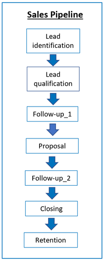  

Normally I would recommend that different types of content to be used in different stages of the sales pipeline, to take account of the varying levels of client/prospect engagement with the vendor’s products and other factors.   Moreover, the mix of content would reflect the vendor’s sales priorities – for example, qualifying prospects vs. increasing contract closure or contract renewal rates.  However, these are far from normal times.  Everyone is very much in “scramble mode”.  Impactful content during the age of the pandemic will add value at most stages of a vendor’s pipeline and meet the overarching goals of maintaining a dialog with clients and prospects, closing sales where possible, and keeping the contract renewal rate up. 
​
Practitioners will note that my version of the pipeline has more emphasis on client follow-up steps.  This reflects my experience that to be successful, vendors of complex B2B products need to take a high touch approach that keeps prospects engaged by frequent demonstrations of product value.  In an upcoming series of posts I will delve into such issues, as well as what sorts of content work best for different pipeline stages, and why.

Credit rating agencies have been called a lot of things over the years, but “dodgy boilers” (per a recent article the Financial Times) has to be a new one.  The journalist leaned into the simile because just as a faulty boiler can blow up a house, so can the prevailing flawed (in his view) rating agency business model destroy the global financial system. 
 
The article revisits familiar topics such as the conflicts of interest allegedly embedded in the agencies’ business structure, whereby issuers pay for their own ratings, and the performance of the US subprime mortgage market during the 2008 financial crisis, when many highly rated issues defaulted. 
 
Such topics have been argued over for years, and we see no profit in relitigating them.  But we do object to two other statements in the article.  The first is that “rating agencies essentially use backwards-looking methodologies”.  The second is that “investors will continue to put blind faith in agencies’ credit ratings”.  Both beliefs have been around for a long time, and both are wrong.  We think that an improved understanding of these points helps to clarify the roles of rating agencies and institutional investors in the debt markets.   It can also help set expectations of their performance in future downturns.  

Credit ratings: “The best lagging indicators on Wall Street”?
That ratings are backwards looking is accepted as an article of faith by many market participants.  There are many reasons for this, but an often-cited cause is that ratings move much more slowly than market-based metrics such as credit spreads, giving rise to the agencies’ unwelcome sobriquet of being of “the best lagging indicators on Wall Street’”.  But to borrow a concept from the tech world, this is a feature, not a bug.  That is, rating systems are managed so that changes in the metrics are directionally correct, with few “reversals”, i.e., when ratings are lowered and then raised quickly, or vice versa.  Ratings were never intended to move ahead of, or lead, markets, although this can happen.  By contrast, market-based metrics, like markets themselves, react quickly to news and are much more volatile.   Both systems have been used for years by investors and risk managers, albeit in different ways that reflect their different performance characteristics. 
 
What ratings do and don’t do
The major agencies have long published statistics on default rates per rating category over different time horizons.  As we will see, these give lie to the idea that ratings are backwards looking. 
 
Before getting into the details, it’s worth recalling that credit ratings claim to do essentially only one thing, namely rank order default risk.  Entities rated, say, single-A should default at a lower rate than those rated BBB, and BBB rated companies should default at a lower rate than those rated BB, and so on.   This construct allows for the possibility that highly rated entities will default (who can forget Lehman Brothers), but it also follows that such events should be exceedingly rare.  This wasn’t the case for the highly rated structured finance assets that defaulted during the financial crisis, but it’s held true for ratings assigned to “corporate” bonds, i.e., those sold by industrial, utility, and financial entities. 
 
The standard methodology for determining default rates begins by grouping entities into rating categories at a given point in time.  The next step is to calculate how many defaulted in the following years, regardless of any subsequent rating changes.  So to determine the average single-A five year default rate, an agency buckets all single-A names together on, say, January 1, 2013, counts the number that defaulted between then and December 31, 2017, and divides the count by the number of companies in the group (or “cohort”) at the beginning of the period (after adjusting for withdrawn ratings and the like).  Default studies cover many years so thus consist of many individual cohorts.  The end results of the studies are cumulative default rates, expressed as percentages, for different rating categories and time horizons, with each default rate reflecting the average experience of its constituent cohorts.  A crucial point, which we touched on above, is that in most cases issuers will have been downgraded many times before they default, but are still grouped according to the ratings they had when their cohorts were formed.    

The punchline is that average cumulative default rates per rating category exhibit the desired pattern of higher default rates on lower rated companies.  This holds over calculation horizons varying from five years (Figure 1a) to 10 and 20 years (Figures 1b and 1c).  Such outcomes, particularly over extended time horizons, are scarcely consistent with the claim that ratings are backward looking metrics.  Indeed, only by being forward looking can any risk measurement scale get these sorts of results.    

Figure 1a: Five-year ave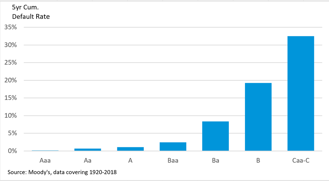rage cumulative default rates per rating category (1920-2018)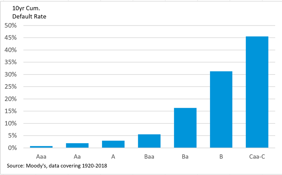

​Figure 1c: 20-year average cumulative default rates per rating category (1920-2018)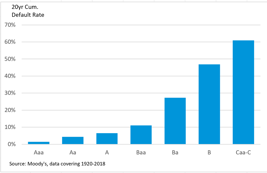

Default rates per rating category can also be measured dynamically, as we do in Figure 2.  Most of the time lower-rated issuers defaulted at higher rates, and this for data spanning almost a century.  The periods when this pattern was violated, mainly during the 1960s, were times with a relatively small number of rated entities and a very limited number of defaults.  

Figure 2: One-year default rates by rating category, 1920-2018 (five-year moving averages)

Institutional investors can, and do, make their own decisions  
We now turn our attention to the claim that “investors will continue to put blind faith in agencies’ credit ratings”.   The corporate bond market is dominated by institutional players.  Such investors are broadly divided between passive asset managers who track ratings-based indices, and active managers who select bonds that they believe are attractive and reject those they believe will underperform.  Passive mangers follow ratings-based benchmarks, so by definition “put blind faith in agencies’ credit ratings”.  As for active managers, they are certainly aware of ratings: if nothing else, they usually can only buy bonds with certain ratings.  They are also consumers of ratings-related research produced by the agencies.  But it is not true that they rely blindly on ratings, something that is evident from bond prices. 
 
Corporate bond investors are intensely focused on the risk of credit deterioration and default.  This makes their assessment credit risk – which is what ratings also provide – a dominant driver of corporate bond prices.  If institutional investors “put blind faith in ratings”, then issues with similar maturities sold by entities in the same sector and with the same rating should trade at very similar prices.  But we find the opposite: prices vary a lot among issues that are otherwise equivalent.  Moreover, the distribution of prices is skewed towards the low side, which is exactly what we’d expect from a decision-making process that focuses on downside risk in the form of credit deterioration and default. 
 
We conclude by returning to the sorry tale of subprime structured residential real estate bonds.  Well before the financial crisis hit, AAA rated subprime bonds traded at substantially cheaper prices than non-subprime issues that were otherwise equivalent (including their ratings).   Thus, even before the crash investors had drawn the conclusion that equally rated subprime and non-subprime bonds did not have equivalent risk levels, although with the benefit of hindsight it is clear that most bondholders underestimated how bad things would get.  This is one area, at least, where investors and the rating agencies have found common ground.

A recent Financial Times article on fixed income exchange traded funds (ETFs) explored at length how portfolio trading has enabled the rapid growth of bond ETFs.  However, while it highlighted, we believe correctly, the implications for liquidity and dealer profitability, it didn’t mention another risk for the market.  This is the potential increase in the mismatch between the performance of many broad market ETFs and the indices that they pledge to track.  If investor expectations in this regard are not met – and we think there’s a good chance this will be the case for many ETFs -- the implications for investors and fund sponsors could be significant.  These include unwelcome attention from regulators, a loss of assets under management, and greater industry concentration.  

​The interplay between fixed income ETFs and portfolio trading
Over the past several years advances in pricing and technology have boosted the ability of specialist firms to price and trade bonds together as blocks, or portfolios.  In this regard the bond markets are catching up with their equity counterparts, where portfolio trades have long been the norm.  It’s a timely development in the world of fixed income, since the rise of ETFs (Figure 1) has increased the demand by investors to trade in and out of the funds with minimal costs. 
​
Figure 1: Growth in global fixed income ETFs ($ trillion)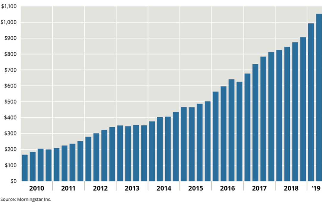

At the heart of the relationship between bond ETFs and portfolio traders is that the latter create and redeem shares in the former via block trades.  This process is common to all ETFs regardless of asset type, of course, and the process in the equity markets (where ETFs have a long history) is often cited as a precedent for bonds.  However, “The equity market as a model for fixed income” analogy falls short in some important ways. 
 
The haves and the have nots: increased bifurcation in bond liquidity
The biggest one is liquidity.  While liquidity varies by company in the equity markets, two-way trading exists in all shares in the leading indices.  So the block trades that create and redeem ETF shares usually contain all the constituents in the ETF and its index.  Not so for corporate bonds, where the gap between liquid issues (mostly larger and sold more recently) and illiquid ones (smaller and older) has plagued the market since its inception.  Reflecting this, ETF-related portfolio trades typically involve around 100 of the most liquid securities.  To provide some context, broad market US investment grade bond indices have over 6,000 securities.  The Vanguard Total Bond Market Fund (BND) ETF cited in the writeup contains in excess of 9,000 issues.
 
The growth of ETFs and improved technology means that portfolio trading is likely to grow in the future, with the probable result that market activity will become concentrated in an ever-smaller group of securities.  This will in turn raise issuance and transaction costs for smaller entities.  Over time, this could lead them to being shut out of the market, leaving the field to larger and more established players
 
The dangers of increased tracking error
We now turn our attention to another concern, that of the impact of portfolio trading on the ability, or inability, of bond ETFs to track closely the performance of their target indices.  This is not a trivial issue: as noted at the outset, when an investor buys shares in an ETF that’s advertised as representing an index, say one for the US investment grade market, they expect to get that performance.  But as we explain below, the use of portfolio trades to create and redeem securities means that in the future this might no longer be true for many funds.    

To be clear, we believe that the performance of the larger and long-established bond ETFs should not be affected by the trend towards portfolio trading. This is because they usually contain most, if not all, of the bonds in their indices.  In this they are helped by the fact that in many cases their benchmarks only include large issues, and thus have fewer bonds.  And over time, these older funds have been able to use the new issue market, which is typically more liquid, to secure bonds that are in their indices.  So when they create and redeem shares through portfolio trades with small numbers of securities, it shouldn’t affect their ability to track their indices with a small amount of performance variation.  That’s because the subset of bonds bought and sold to represent the ETF matches the issues and their weights in both the fund and its target index.

The problem arises for ETFs and mutual funds that contain only a subset of the bonds in their target benchmarks, but that are intended to follow the performance of the broad benchmarks with minimal variation.  The managers of such funds, which are often smaller and newer, have chosen not to “buy the market”, or at least have not yet had the opportunity to do so.  Instead, the portfolios of liquid bonds that they hold are selected to track their broad market indices with minimal forecast variation, or “tracking error volatility”, to introduce an industry term.   This usually doesn’t create problem for liquid sectors, for example Treasury securities.  But it does for less liquid ones, principally corporate bonds.  And that, unfortunately in this regard, is where most of the activity has been (Figure 2). 
​
Figure 2: Inflows into US ETFs and Mutual Funds by Sector (source: IMF, Lipper)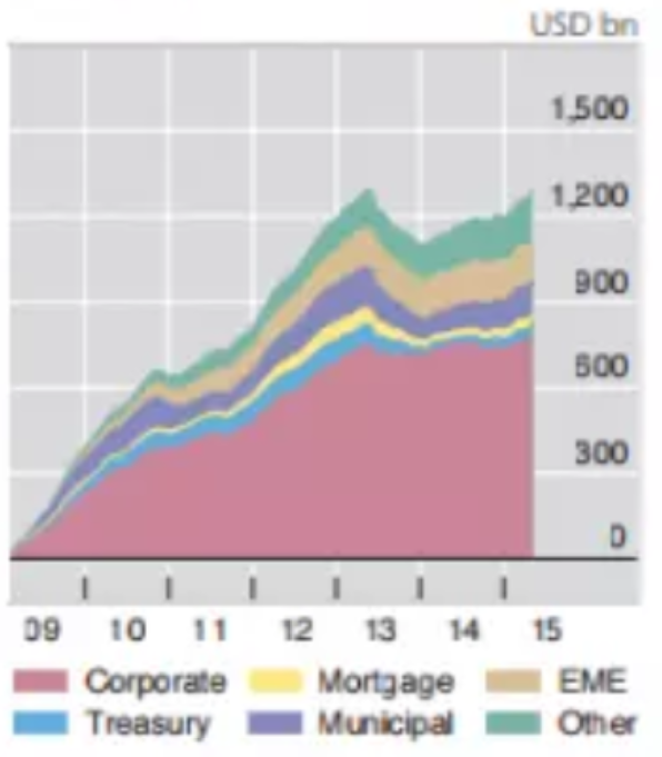

​
​Potential regulatory and investor reactions
Regulators have been taking an increasingly dim view of financial products that do not perform as promised.  So should the increased use of bond portfolio trading cause a deviation between the performance of an ETF and the index it’s supposed to track, we would not be surprised to a similar development here.  Moreover, as we described in an earlier post, investors have shown themselves to be quite willing to take their business elsewhere if they are disappointed in the performance of a financial product.  We believe that the latter development would lead to further growth of the leading ETFs and fund sponsors, squeezing out the smaller players and thus reducing the scope for innovation and competition.  

A recent Financial Times article featuring the juggernaut known as Vanguard Asset Management provided a useful reminder, if we needed one, of the declining business outlook for US active asset managers.   It’s a sad but familiar tale, particularly in the equity space.  Yet despite the negative trends which we touch on later, the sector doesn’t seem to be exhibiting signs of severe crisis.  Yes, equity valuations are down and the rate of consolidation is up, but there are few indication of similarity to the proverbial buggy whip business at the dawn of the automobile era. 

In this article we review some key, mostly negative, trends for US active asset managers and why many players have been able to maintain their business models in the face of these pressures.  We then suggest a path forward for them, one that we’ll explore in greater length in an upcoming post.

The money flows out, the fee levels go down
It’s never good when your clients are “voting with their feet”, and are doing so against you.  This is been the case for active asset managers in the US, who have experienced fund outflows in excess of $2 trillion during the past decade.  By contrast, over the same period passive management strategies have seen inflows of close to $3 trillion (Figure 1). 

Figure 1: US fund flows by investment style (2010-2019)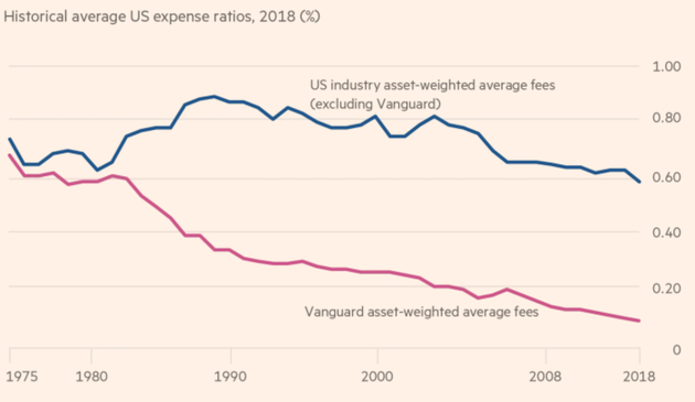

The decline in active management fees as expressed as a percent of assets under management, or AUM (Figure 2) is a much-cited headline development, and one that only compounds the problem.  The Figure shows an even sharper drop in passive fee levels.  But this is from a much lower base, so the decline in the dollar value is less. 
​
Figure 2: AUM fee trends, 2013-2018

In most industries the loss of a significant portion of a core business and a double-digit drop in the price for your product would be classified as an existential crisis.  Not so – or at least not yet -- for US active asset managers.  So what’s going on?
 
A rising tide floats most boats
The main reason that relative calm prevails is the buoyant stock and bond markets over the past decade, a period during which the S&P 500 Index posted a gain of 187% and the cumulative total return for investment grade bonds was 65%.  This means that rises in market values have more than offset fund outflows, leading to substantial gains in assets under management held by fund managers.  Which are, of course, the basis for their fees.  Indeed, in many cases the increase in value has been more than enough to counter the fall in AUM fees, expressed as a percentage of funds under management. 
This dynamic is illustrated in Figure 3, which shows the breakdown of public assets held in US mutual funds and exchange traded funds and their totals between 2008 and 2018.  Even though the actively managed share of public assets fell from 82% to 64%, the nominal amount rose from $5.2 trillion to $11.5 trillion, more than offsetting the fall in fee levels (expressed as a percent of AUM) over the period. 
​
Figure 3: US AUM split by style and vehicle, 2008 and 2018 (Source: ICI)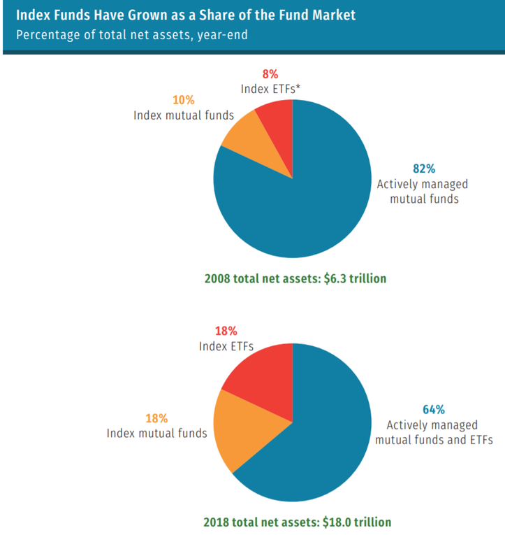

There’s no reason to change – yet
There are other reasons why the active management businesses remain attractive for fund managers.  One is the sheer size of the sector: active management fees make up around a quarter of revenue for US asset managers.  Secondly, while active management fees expressed as percent of AUM have declined, they remain a lot higher than for passive strategies – where fees are also down sharply.   Thirdly, the leading players have extensive infrastructures, relationships with distributors of their products, and brand equity in the form of reputations for client service and alpha generation (even if the latter has taken hits recently) that they are loath to abandon. 

Finally, we should never underestimate the inertia inherent in any large organization, along with the logic that there’s no need to make radical changes to a model that’s still producing good results.  Lending support to the latter point, average asset manager revenue growth and margin levels compare quite favorably to those in other banking/finance sectors (Figure 4).
​
Figure 4: Asset management revenue growth and margins vs. other financial sectors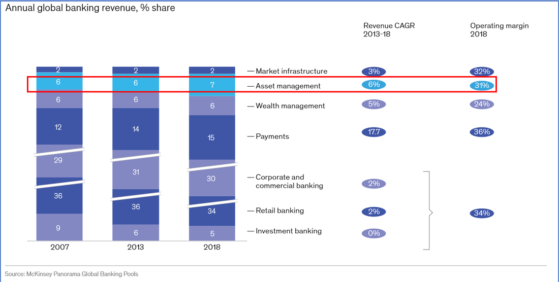

What goes up must “correct”, eventually
As always, the past is not prologue for the future.  In the case of asset managers, markets will fall, as they always do, at which point the deteriorating business fundamentals for active strategies will be laid bare. 
 
To make matters worse, fund managers’ expenses has been climbing (Figure 5).  The Figure highlights a couple of trends that in particular bode ill for asset managers in the future.  The first is that the fastest growth is occurring in expenses related to areas other than “Investments”.  Thus, the “tooth-to-tail” ratio – to borrow a term from the military – is declining.   That is, the amount of resources going into the parts of the business that directly generate revenue (the “teeth”) is falling relative to the other areas that do not (the “tail”). 
 
The second trend is that the estimated average costs in relation to AUM have fallen slightly since 2007 (from 26 bp to 24 bp), as the growth in nominal assets has outpaced the rise in expenses.  When markets sell-off and AUM declines, this expense ratio will rise, unless managements take some pretty drastic steps. 
 
Figure 5: North American asset management costs by function (2007-2018)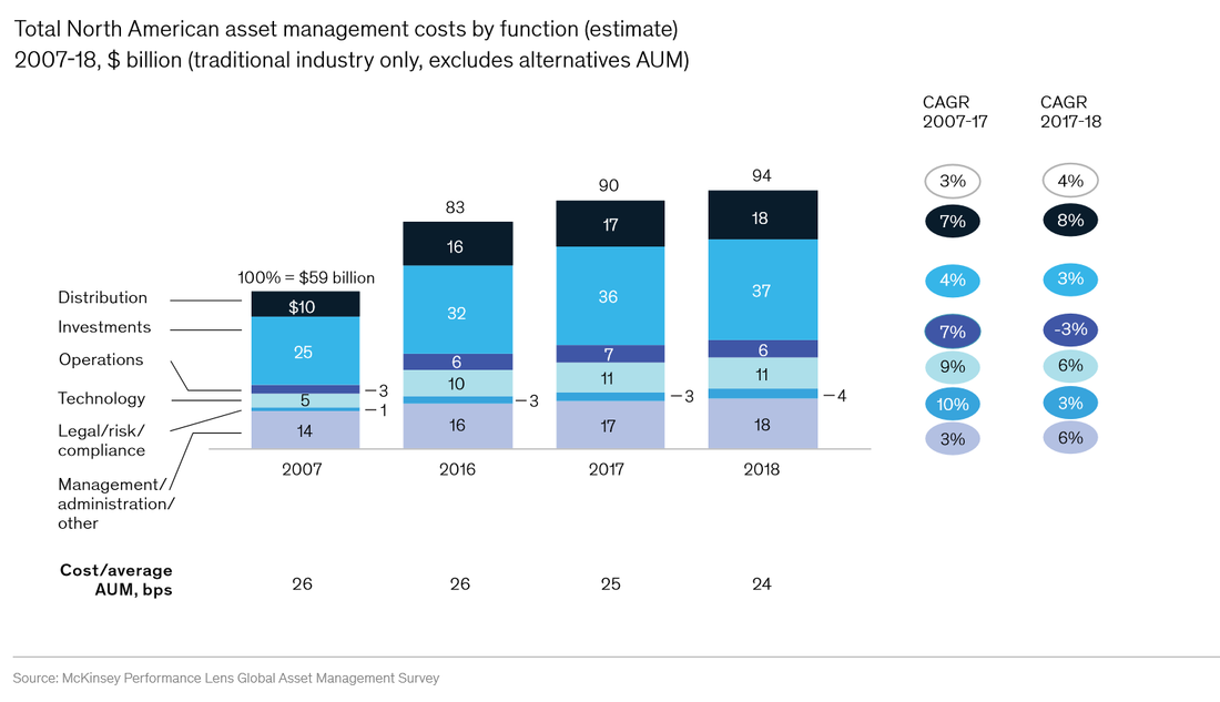

​Alpha Lite: a proposed solution to the conundrum
Of course, the leaders of big asset managers are well aware of the foregoing trends.  One response has been to seek new ways to generate alpha, often in the form of spending on alternative data and artificial intelligence, in particular machine learning (these trends are one of the drivers of the increased spending for Technology in shown Figure 5).  But such strategies require heavy investments in data, systems, and headcount, and have uncertain payoffs. 
 
We suggest an alternative approach, one that allows active asset managers to preserve their business models, and thus fees, while leveraging their human capital in the form of portfolio managers and analysts.  This is to integrate quantitative entity and security-level relative value and risk signals into their existing processes.  This “alpha lite” approach has been around for a while, but we believe it deserves an even closer look now.  We will explore it in detail in an upcoming post.